
Normandie On Sea is the perfect little gem with the ocean on your doorstep, spectacular views and an incredible location, walking distance to restaurants, supermarkets and art galleries.
Your Hermanus Home away from Home. If you want to unwind and escape your daily routine, Normandie On Sea has everything you’ll need to have the perfect holiday or break close to the most southern tip of Africa- the whale capital of the world.
A seafront self-catering abode with warm and homey spaces and equipped with everything you will possibly need.
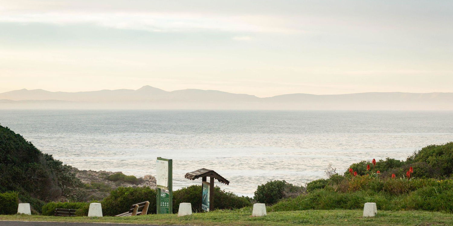
The Famous Hermanus Cliffpath and Ficks Pool is just across from Normandie. And if you want to stay home and order in, you can still do whale watching straight from the living room!!!
We are looking forward to your stay with us!
Share This Page